3 Data
3.1 Sources and coverage
The analysis uses a balanced monthly panel covering January 2000 to January 2026, 313 observations, with no missing months and no missing values in any series. Quantity and generation series are drawn from the Energy Administration’s Energy Statistics Query System (Energy Administration, Ministry of Economic Affairs, 2026): fossil fuel imports by country of origin and coal type, renewable and nuclear electricity generation, electricity consumption, and the aggregate energy indicators. The exchange rate is the Central Bank’s monthly average of the New Taiwan Dollar against the US Dollar (Central Bank of the Republic of China (Taiwan), 2026). International fuel prices are taken from the World Bank Pink Sheet (World Bank, 2026).
3.2 Measuring fossil fuel imports
Three measurement decisions materially affect the answer and are therefore stated explicitly.
Common energy units. The three import series are reported in incommensurable physical units: coal and liquefied natural gas in tonnes, crude oil in thousand barrels. They cannot be added directly. All quantities are therefore converted to terajoules using the net calorific values published by the Energy Administration (Energy Administration, Ministry of Economic Affairs, 2024), with one kilocalorie taken as \(4.1868 \times 10^{-6}\) GJ, consistent with that table’s own convention that one kilogram of oil equivalent equals 10,000 kcal. The values applied are 5,846 kcal/kg for imported steam coal for power generation, 4,710 kcal/kg for sub-bituminous coal for power generation, 7,010 kcal/kg for imported coking coal, 7,415 kcal/kg for anthracite, and 8,613 kcal per litre for crude oil.
Liquefied natural gas is the one exception. The official table quotes 8,710 kcal per cubic metre of regasified gas, a volume basis, whereas the import series records the mass of liquefied gas landed. Converting tonnes of liquid to cubic metres of gas requires a regasification factor the table does not supply, so LNG retains the international mass-basis convention of approximately 52 GJ per tonne, which lies within the standard 48–54 GJ/t range. This is the largest single residual measurement uncertainty in the dependent variable — see the discussion of limitations in Section 6.4.
Restricting to power-sector fuels. The research question concerns electricity generation, but total fossil fuel imports are dominated by fuels that are not burned for power. Crude oil accounts for 38–55% of imported fossil energy across the sample yet is refined largely for transport and petrochemical feedstock; coking coal is consumed by the steel industry. Including them injects variation unrelated to the power sector, biasing the estimated elasticity toward zero and inviting a spurious reading in favour of the additionality paradox. Fortunately the source data disaggregate coal by type, which permits a clean separation. The primary dependent variable is therefore
\[ FFI^{power}_t = \text{steam coal}_t + \text{sub-bituminous coal}_t + \text{LNG}_t, \]
measured in terajoules, with the all-fuel aggregate \(FFI^{all}_t\) retained as a robustness check. Within \(FFI^{power}\), the LNG share rose from 35.9% in 2016 to 52.5% in 2025 while the steam coal share fell from 52.6% to 40.2%, so the composition of the dependent variable is itself shifting over the transition period.
Shipment lumpiness. Monthly import data are driven partly by vessel scheduling rather than by economic conditions. The first difference of \(\ln FFI^{power}\) exhibits a first-order autocorrelation of \(-0.35\), and the corresponding figure for crude oil is \(-0.49\); aggregating to quarterly frequency reduces it to \(-0.01\). This mean-reverting noise is not an economic signal, and it is accommodated in two ways: the distributed-lag structure of the ARDL absorbs it within the monthly specification, and a quarterly specification is estimated as a robustness check.
3.3 Renewable generation and the choice of sample period
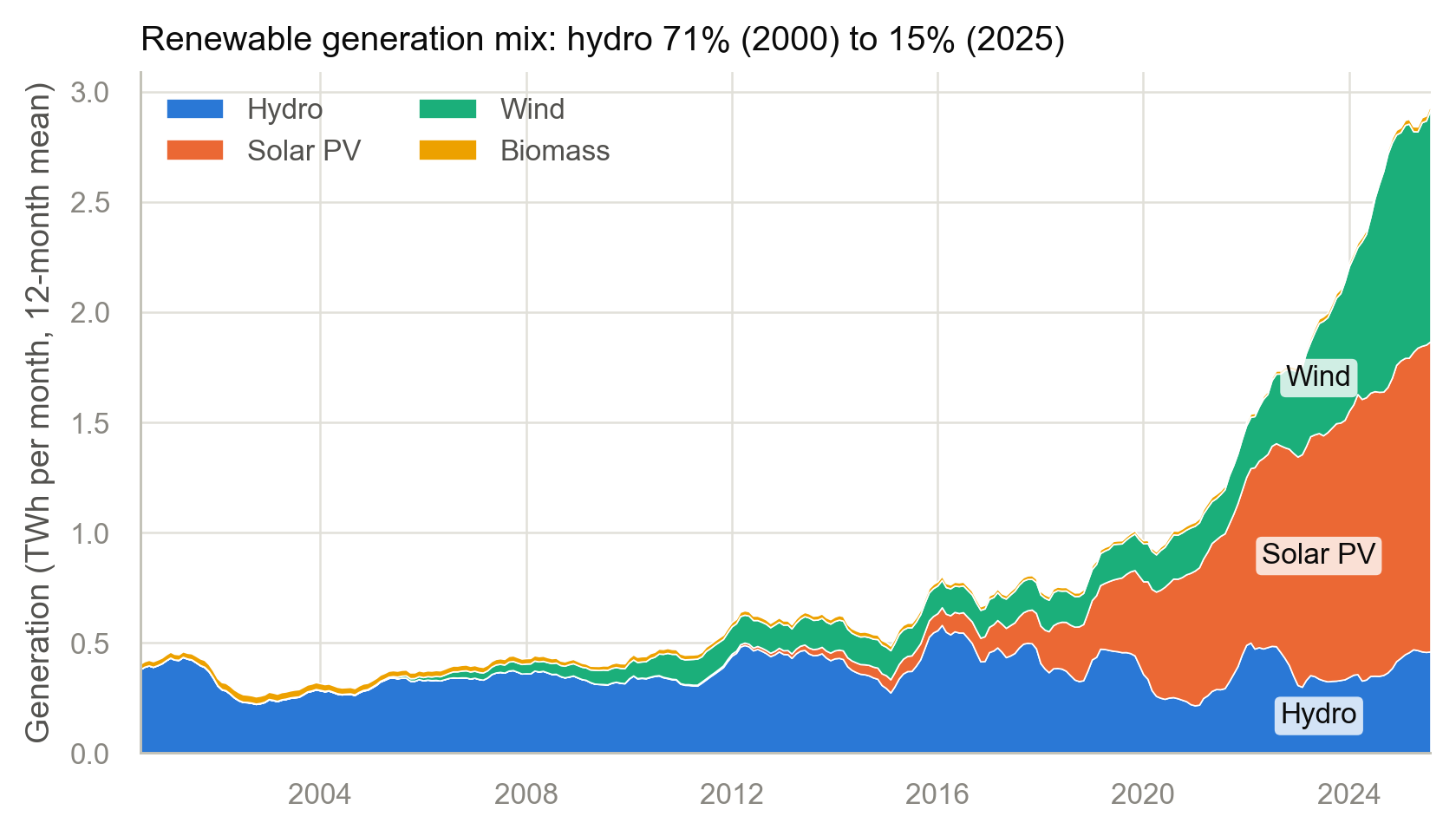
The composition of renewable generation changed fundamentally over the sample. Hydropower accounted for 71.8% of renewable output in 2000 but only 14.3% by 2025, while solar photovoltaics and wind rose from zero to 43.4% and 31.6% respectively (Figure 3.1). Early-sample renewable generation is therefore essentially a function of rainfall, which is climate-driven and dispatchable; late-sample renewable generation is policy-driven and intermittent. These are not the same economic mechanism, and a single elasticity estimated across the whole period would not have a stable interpretation.
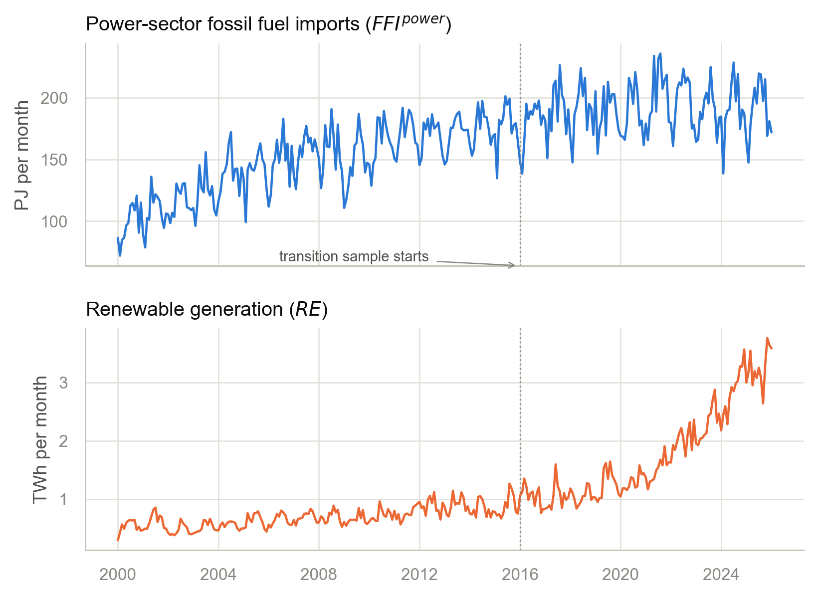
Three considerations lead to January 2016 as the start of the primary sample. It coincides with the launch of the transition policy package; solar and wind generation are strictly positive throughout, permitting logarithmic transformation that is unavailable for eleven months of 2000; and the partial correlation between the seasonally adjusted and detrended residuals of \(\ln FFI^{power}\) and \(\ln RE\) is \(-0.29\) from 2016 onward against \(-0.01\) before 2016, indicating that whatever displacement signal exists is concentrated in the later period. The full sample from 2000 is retained as a robustness check. Over the transition sample, renewable generation tripled, from a monthly mean of 1.06 TWh in 2016 to 3.22 TWh in 2025, while power-sector fossil fuel imports rose by 6.3%, from 179.2 PJ to 190.6 PJ per month. Figure 3.2 presents both series.
3.4 Control variables
Electricity consumption (\(EC_t\)) is aggregate consumption in MWh, spliced from two source files that partition at December 2017. The splice requires no level adjustment: year-on-year growth at the junction is \(+0.48\%\) and \(+5.51\%\), well inside the sample distribution with mean \(+2.04\%\) and standard deviation \(4.95\%\).
Nuclear generation enters as a share rather than in logarithms. Following the closure of the second Maanshan unit in May 2025, nuclear output is exactly zero in nine months of the sample, so \(\ln(NUC_t)\) is undefined precisely during the most policy-relevant period. The specification therefore uses \(NUC^{share}_t = NUC_t / EC_t\), which retains all 313 observations at the cost of interpreting the coefficient as a semi-elasticity. The nuclear share fell from an annual mean of 0.126 in 2016 to 0.013 in 2025.
International fuel prices. The original design controlled import cost through the exchange rate alone. That is insufficient: the variation in import quantities over 2021–2023 was driven predominantly by price shocks, and omitting prices would load that variation onto the exchange rate coefficient. Taiwan’s own import unit values were considered and rejected on two grounds: they are available only from 2014, and more importantly they are endogenous, reflecting Taiwan’s own contracting structure, purchase timing and freight arrangements, all of which co-move with domestic demand and dispatch decisions. International benchmark prices are exogenous to Taiwan, which is a price taker.
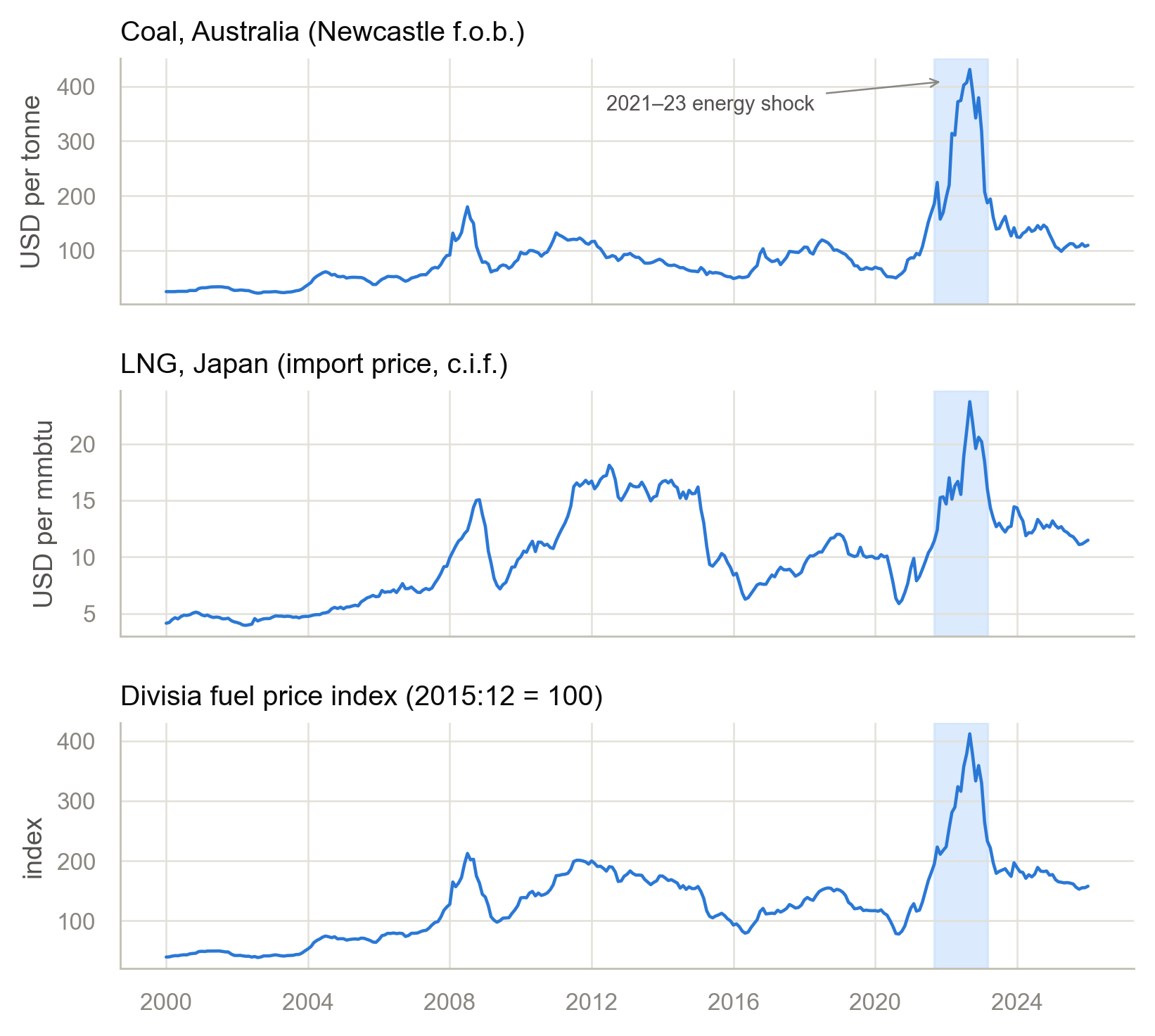
The three Pink Sheet series are selected to match Taiwan’s actual sourcing structure. Australia is consistently the largest coal source, supplying 50.7% of coal imports, so the Newcastle f.o.b. quotation applies. Australia and Qatar together supply 56.4% of LNG over the period, a share rising from 43.6% in 2016 to 67.2% in 2025, and the Japan c.i.f. import price is the established Asian regional benchmark for such cargoes. Middle Eastern producers supply 70.7% of crude oil, led by Saudi Arabia at 31.5% and Kuwait at 18.9%, and these barrels are priced off Dubai. The Henry Hub and WTI series are deliberately not used: gas markets are regionally segmented, the correlation between Henry Hub and Japanese LNG over the transition sample is only \(+0.60\), and in September 2022 Henry Hub stood at 7.76 USD/mmbtu against 23.73 for Japanese LNG.
Because the dependent variable is an aggregate of two fuels, the price control is constructed as a Törnqvist (discrete Divisia) chained index over coal and LNG, with cost-share weights updated each period (Diewert, 1976):
\[ \Delta \ln PF_t = \sum_i \frac{w_{it} + w_{i,t-1}}{2}\, \Delta \ln P_{it}, \qquad w_{it} = \frac{P_{it} Q_{it}}{\sum_j P_{jt} Q_{jt}}, \]
normalized to 100 in December 2015. Figure 3.3 plots the components and the index, which peaked at 411.8 in September 2022 against 92.9 in January 2016.
3.5 An indicator that cannot serve as the dependent variable
The Energy Administration publishes an import-dependence ratio, imported energy over total energy supply, which is verbally identical to the concept in this book’s title. It is not used as a dependent variable, for a reason worth stating because the temptation is real. Over the transition sample its correlation with \(\ln RE\) is \(-0.930\). That figure is an accounting identity, not an empirical finding: renewable output belongs to the denominator’s domestic supply component, so renewable expansion reduces the ratio by construction. Regressing it on renewable generation would deliver a large, highly significant negative coefficient that measures nothing but the definition. The indicator is used here only descriptively, in Figure 1.2, and as a cross-check on the 95.8% figure reported by the Energy Administration.