5 Results
5.1 Integration properties
The dependent variable \(\ln FFI^{power}\) is \(I(1)\) in both samples: the ADF test does not reject a unit root in levels (\(p = 0.42\)), rejects decisively in first differences, and Zivot–Andrews does not reject even when a break is permitted. This satisfies the prerequisite of the bounds test, which requires an \(I(1)\) dependent variable and no \(I(2)\) variables.
The renewable series present mixed evidence. Over the transition sample the ADF test rejects a unit root in the levels of \(\ln RE\), \(\ln RE^{disp}\) and \(\ln RE^{var}\), while KPSS rejects stationarity for \(\ln RE\). The ARDL framework explicitly permits regressors of mixed integration order, so this does not compromise the bounds test. It is also worth noting that the Zivot–Andrews break in \(\ln ER\) falls in February 2022, coinciding with the invasion of Ukraine, which independently corroborates the break specification used below.
5.2 Cointegration
For the primary specification the overall \(F\) statistic is 17.62 against a simulated 99% upper bound of 5.01, so the null of no cointegration is rejected decisively. The simulated critical values are indeed more conservative than the asymptotic ones, 5.01 against 4.45 at the 99% level, which validates the decision to simulate. Critically, all nine specifications reject all three tests of the McNown et al. (2018) protocol, so the rejections are not attributable to degenerate cases.
5.3 Long-run coefficients
The estimated long-run relationship in the primary specification is
\[ \ln(FFI^{power}) = -0.039 \ln(RE) + 0.555 \ln(EC) - 0.480\, NUC^{share} - 0.145 \ln(ER) + 0.047 \ln(PF) . \]
| Regressor | β | SE | p | Reading |
|---|---|---|---|---|
| \(\ln RE\) | −0.0391 | 0.0209 | 0.061 | the elasticity of interest |
| \(\ln EC\) | +0.5551 | 0.1888 | 0.003 | inelastic but firmly significant |
| \(NUC^{share}\) | −0.4795 | 0.1655 | 0.004 | semi-elasticity; sign as expected |
| \(\ln ER\) | −0.1452 | 0.1232 | 0.239 | depreciation dampens imports, not significant |
| \(\ln PF\) | +0.0466 | 0.0116 | <0.001 | small magnitude, discussed in the next chapter |
The central estimate is \(\eta_{RE} = -0.039\). A one percent increase in renewable generation is associated with a reduction in power-sector fossil fuel imports of 0.039 percent. The delta-method interval is \([-0.080, 0.002]\) with \(p = 0.061\), marginally outside conventional significance; the bootstrap interval is \([-0.075, -0.001]\) and excludes zero. Given that \(\eta_{RE}\) is a ratio, the bootstrap interval is the more reliable of the two, and the honest summary is that the elasticity is negative and very small, with significance at the margin of the conventional threshold. The substantive conclusion does not turn on which side of \(0.05\) the \(p\) value falls: an elasticity of \(-0.039\) is economically negligible whether or not it is statistically distinguishable from zero.
The control variables behave sensibly and are estimated far more precisely than the variable of interest. Electricity consumption carries an elasticity of \(+0.555\): demand growth raises fossil fuel imports, inelastically but robustly. The nuclear share carries \(-0.480\), correctly signed, indicating that nuclear output does displace imported fossil fuel. The exchange rate is correctly signed but insignificant.
The error correction coefficient is \(\lambda_1 = -1.653\). Its absolute value exceeds unity, which is addressed as a caveat in the next chapter.
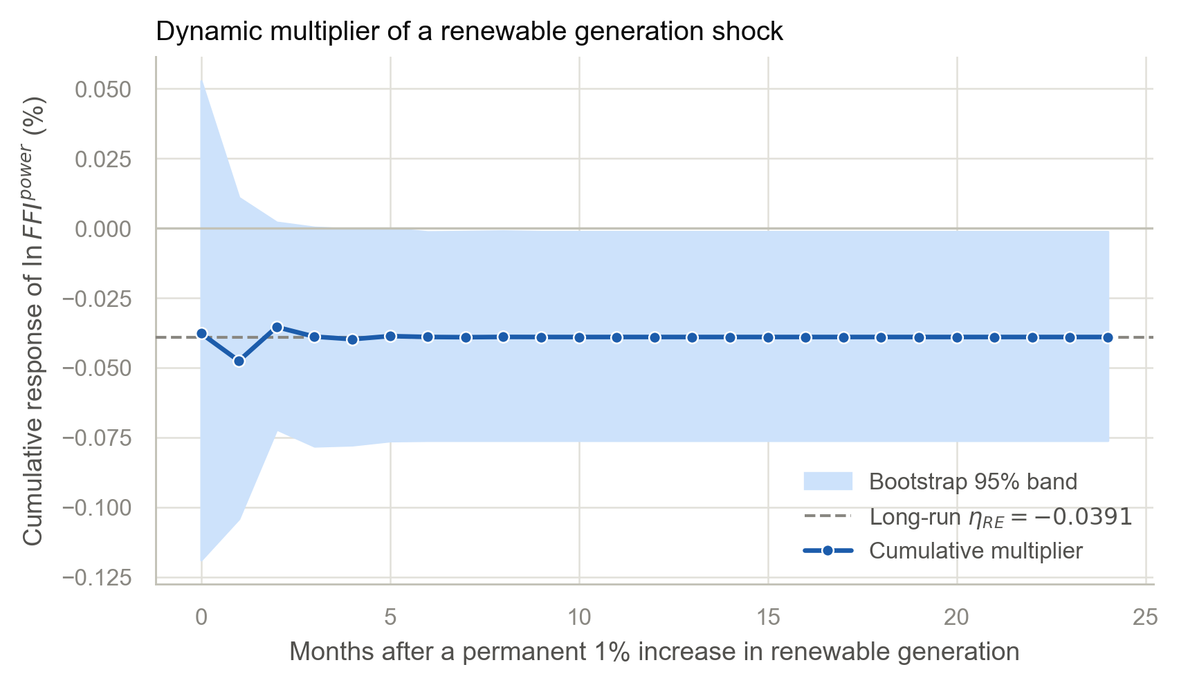
Figure 5.1 traces the cumulative dynamic multiplier of a permanent one percent increase in renewable generation. The response settles within roughly three months and converges to \(-0.0391\), identical to the estimated long-run coefficient, which provides an independent numerical check on the elasticity calculation.
5.4 Diagnostics
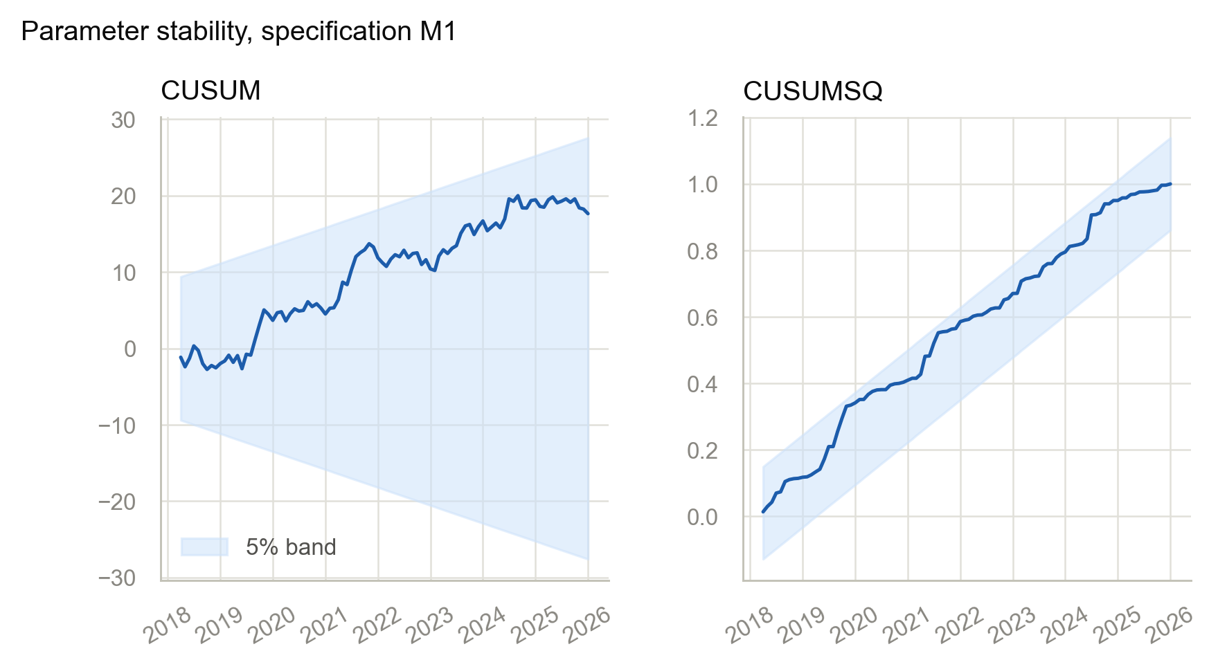
The primary specification passes every test: no serial correlation at twelve lags (\(p = 0.139\)), no ARCH effects (\(p = 0.271\)), normally distributed residuals (\(p = 0.898\)), correct functional form by the RESET test (\(p = 0.652\)), and parameter stability by both CUSUM and CUSUMSQ. Adjusted \(R^2\) is 0.776. One exception should be recorded: the full-sample specification fails the ARCH test at the 5% level (\(p = 0.041\)), which is unsurprising over a 26-year window spanning two energy price shocks and is a further reason to treat the transition sample as primary.
The concern that renewable generation and the nuclear share would prove too collinear to separate does not materialize. Although their correlation in levels is \(-0.767\), the maximum variance inflation factor in the estimated model is only 3.36, because the error-correction model enters the variables as differences and lagged levels rather than as raw levels. Figure 5.2 presents the stability plots.
5.5 Robustness
Table 5.2 collects the elasticity across all specifications. Every specification returns a negative estimate, ranging from \(-0.003\) to \(-0.075\). The bootstrap interval excludes zero in four of the nine point-estimate specifications and includes it in the other five. The estimate is not sensitive to the seasonal specification: replacing eleven monthly dummies with three Fourier pairs moves the elasticity only from \(-0.0391\) to \(-0.0403\). Aggregating to quarterly frequency, which removes the shipment-lumpiness noise, roughly doubles the estimate to \(-0.0739\) and sharpens its significance.
| Spec | Variation | \(\eta_{RE}\) | p | Bootstrap 95% CI |
|---|---|---|---|---|
| M1 | Main: FFI_power, ln RE, 2016+ | −0.0391 | 0.061 | [−0.075, −0.001] |
| M2 | FFI_all (adds crude oil + coking coal) | −0.0375 | 0.221 | [−0.090, +0.016] |
| M3 | Full sample from 2000-01 | −0.0422 | 0.075 | [−0.086, +0.003] |
| M4 | RE split: dispatchable vs. variable | −0.0032 | 0.827 | [−0.032, +0.025] |
| M5 | Drop nuclear share | −0.0228 | 0.374 | [−0.070, +0.023] |
| M6 | Quarterly frequency | −0.0739 | 0.016 | [−0.123, −0.027] |
| M7 | Fourier seasonality (order 3) | −0.0403 | 0.044 | [−0.075, −0.003] |
| M8 | Unrestricted intercept and trend | −0.0754 | 0.010 | [−0.127, −0.025] |
| M9 | Fuel-specific prices | −0.0377 | 0.084 | [−0.076, +0.001] |
Two variants deserve individual attention. Dropping the nuclear control (M5) attenuates the elasticity from \(-0.039\) to \(-0.023\) and renders it insignificant. The direction is exactly what omitted-variable bias predicts: with the simultaneous nuclear phase-out unaccounted for, part of the fossil fuel expansion required to replace nuclear output is wrongly attributed to renewables, pulling the estimate toward zero. Widening the dependent variable (M2) to include crude oil and coking coal degrades the model materially: the electricity consumption coefficient collapses to \(-0.054\) and loses all significance, since electricity demand must raise power-sector fuel imports — direct evidence that the wider aggregate is contaminated by fuels unrelated to electricity generation.
5.6 Decomposing renewables: the intermittency mechanism
Splitting renewable generation into dispatchable sources (hydropower, biomass, waste incineration and geothermal) and variable sources (solar and wind) produces the clearest finding in the study. The partition is exhaustive: dispatchable plus variable generation sums to the total.
| Coefficient | SE | p | |
|---|---|---|---|
| Dispatchable renewables | −0.0373 | 0.0235 | 0.112 |
| Variable renewables | −0.0032 | 0.0145 | 0.827 |
Dispatchable renewables display a displacement effect roughly 11.7 times larger than variable renewables, and the coefficient on solar and wind is indistinguishable from zero. Precisely the technologies at the centre of Taiwan’s transition policy, and the ones that grew fifteen-fold and eight-fold respectively between 2016 and 2025, are the ones with no measurable effect on fossil fuel imports.
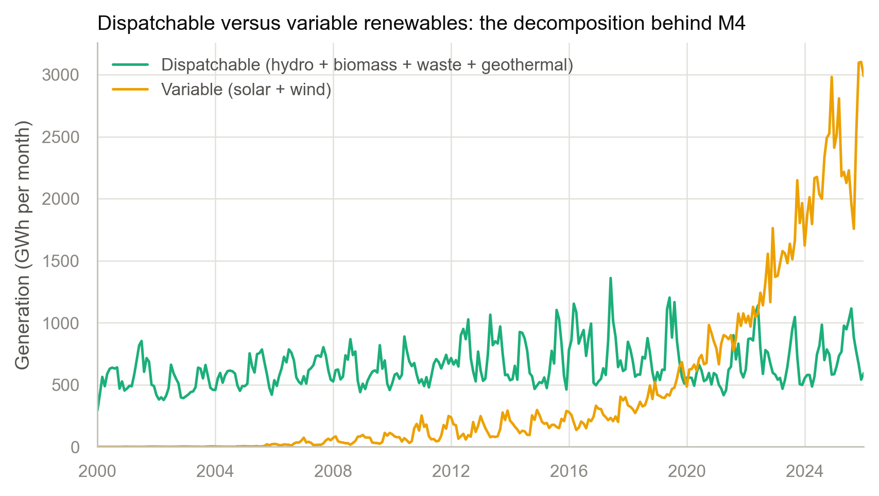
This replicates Marques et al. (2018) in a setting they did not examine. Their European sample retained cross-border balancing capability; Taiwan’s grid has none, so intermittent output must be backed by domestic reserves that remain fuelled by imports regardless of how much solar and wind capacity is added. The result is therefore not merely a robustness check but the mechanism underlying the aggregate finding.
5.7 The elasticity is a recent phenomenon
Figure 5.4 plots \(\eta_{RE}\) estimated over rolling 96-month windows. The estimate was significantly positive, at \(+0.19\), in windows ending around 2010–2011, declined steadily thereafter, and turned negative only after approximately 2022, reaching \(-0.051\) at the end of the sample.
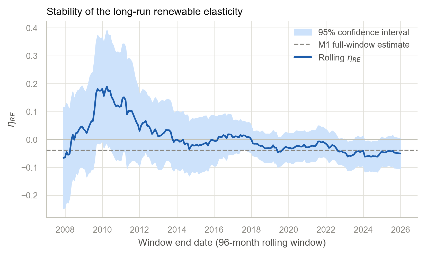
The positive early estimate is interpretable rather than anomalous. In that period renewable generation was overwhelmingly hydropower and was expanding alongside rapidly growing electricity demand, so renewable output and fossil fuel imports rose together: energy addition in its purest form. The transition to a negative elasticity coincides with the point at which solar and wind capacity became large enough to affect dispatch. This provides empirical justification for treating 2016 onward as the primary sample, rather than merely a convenience dictated by data availability.